原 AMSS-NCKU 程序由 C++ 与 Fortran 混合开发,使用时需要手动编译、手动设置输入文件、手动运行多个可执行文件,并借助第三方软件(GnuPlot、Mathematica、Matlab、Python 等)绘图,操作较为繁琐。重庆理工大学团队利用 Python 对 AMSS-NCKU 进行了进一步开发,将原有操作流程尽可能自动化,完成了用户友好型界面,支持 Python 命令行运行与 Jupyter Notebook 运行两种方式。
两种运行方式
Python 命令行运行
编辑输入脚本 AMSS_NCKU_Input.py 后,在终端执行一条命令即可启动整个模拟;程序内置交互式模块,会在计算前检查网格层级、分辨率等参数并给出引导提示,方便初学者使用。
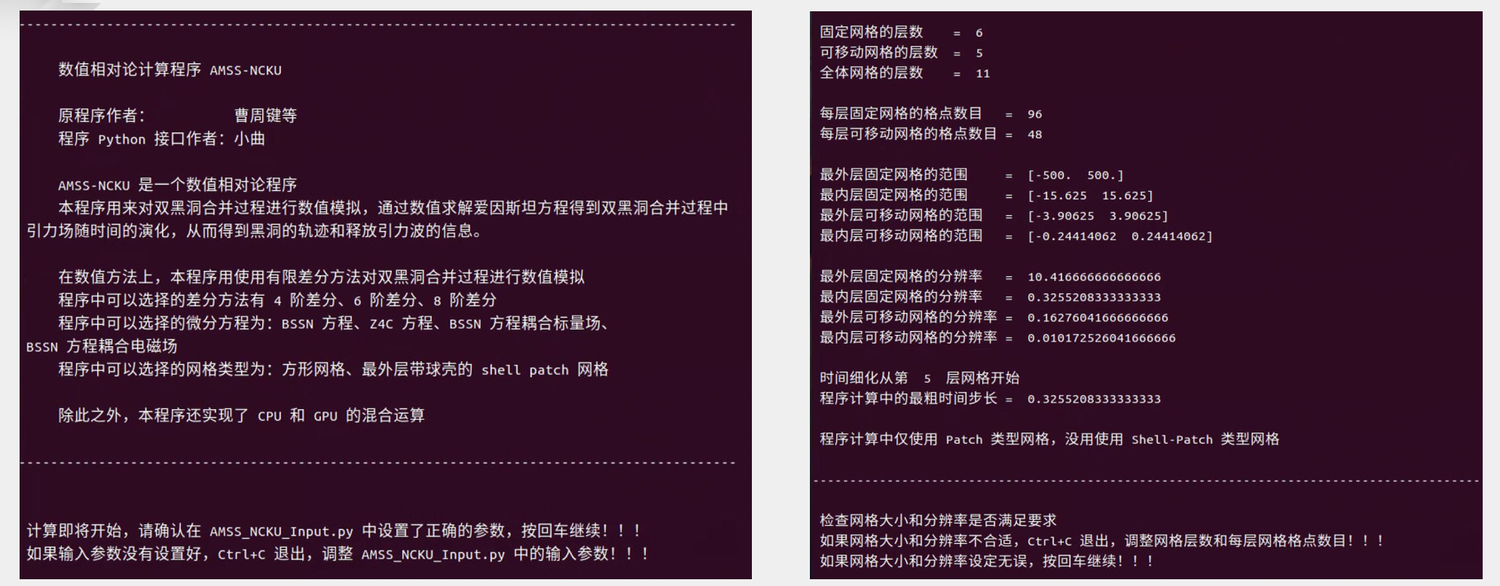
Jupyter Notebook 运行
界面同样支持在 Jupyter Notebook 中逐单元运行:用 %%writefile 魔术命令生成 AMSS_NCKU_Input.py,依次执行初始化、参数设定、启动计算与结果绘图的代码单元。
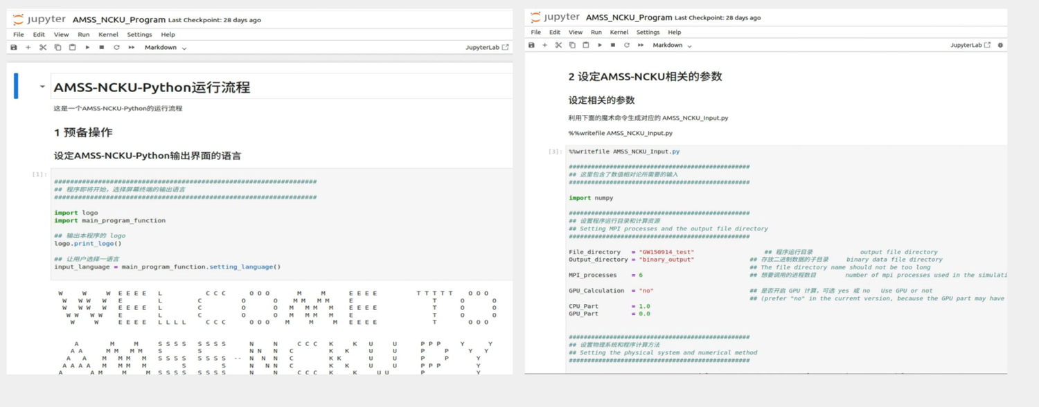
一个输入脚本
用户在 AMSS_NCKU_Input.py 中指定黑洞系统的基本物理输入(质量、电荷、自旋、初始位置与轨道动量)以及数值方法与网格设置(计算方程形式、有限差分阶数、网格层数与格点数):
以下为 GitHub 最新版的完整输入脚本(另提供 Jupyter Notebook 版本 AMSS_NCKU_Input.ipynb):
#################################################
## 这里包含了数值相对论所需要的输入
#################################################

import numpy

#################################################
## 设置程序运行目录和计算资源
## Setting MPI processes and the output file directory
#################################################

File_directory   = "BBH_test_GW150914"            ## 程序运行目录             output file directory
Output_directory = "binary_output"               ## 存放二进制数据的子目录     binary data file directory
                                                 ## The file directory name should not be too long
MPI_processes    = 4                             ## 想要调用的进程数目        number of mpi processes used in the simulation
OMP_processes    = 4                             ## 想要调用的线程数目        number of OpenMP threads per MPI process
cores_per_numa   = OMP_processes                 ## number of CPU cores per NUMA node (for processor binding)

GPU_Calculation  = "no"                          ## 是否开启 GPU 计算,可选 yes 或 no   Use GPU or not
                                                 ## (prefer "no" in the current version, because the GPU part may have bugs when integrated in this Python interface)
CPU_Part         = 1.0
GPU_Part         = 0.0


#################################################
## 设置物理系统和程序计算方法
## Setting the physical system and numerical method
#################################################

Symmetry                 = "equatorial-symmetry"   ## Symmetry of System: choose equatorial-symmetry, no-symmetry, octant-symmetry
                                                   ## 注意:如果选择 octant-symmetry 最好使用固定网格计算,octant-symmetry 对移动网格有些 bug
Equation_Class           = "BSSN"                  ## Evolution Equation: choose "BSSN", "BSSN-EScalar", "BSSN-EM", "Z4C"
                                                   ##       BSSN 和 Z4C   适合于 GR 旋转黑洞的真空计算
                                                   ##       BSSN-EM      涉及 GR 带电黑洞的真空计算
                                                   ##       BSSN-EScalar 涉及到标量张量-F(R) 理论的计算,需要在后面设定额外参数
                                                   ## 注意:GPU 计算仅支持 BSSN      GPU calculation only supports "BSSN"
                                                   ## 这里选择 BSSN-EScalar,需要在后面设定 F(R) 理论的参数
                                                   ## If "BSSN-EScalar" is chosen, it is necessary to set other parameters below
Initial_Data_Method      = "Ansorg-TwoPuncture"    ## 设置求解数值相对论初值的方法
                                                   ## initial data method: choose "Ansorg-TwoPuncture", "Lousto-Analytical", "Cao-Analytical", "KerrSchild-Analytical"
                                                   ## 注意:当前 BSSN-EM 的计算不支持用解析公式 Lousto-Analytical、Cao-Analytical、KerrSchild-Analytical
                                                   ##       当前 BSSN-EScalar 的计算不支持用解析公式 Lousto-Analytical、Cao-Analytical、KerrSchild-Analytical
Time_Evolution_Method    = "runge-kutta-45"        ## 时间演化方法     time evolution method: choose "runge-kutta-45"
Finite_Diffenence_Method = "6th-order"             ## 有限差分方法     finite-difference method: choose "2nd-order", "4th-order", "6th-order", "8th-order"


#################################################
## 设置时间演化信息
## Setting the time evolutionary information
#################################################

Start_Evolution_Time     = 0.0                    ## 起始演化时间   start evolution time t0
Final_Evolution_Time     = 1000.0                 ## 最终演化时间   final evolution time t1
Check_Time               = 100.0
Dump_Time                = 100.0                  ## 每隔一定时间间隔储存数据   time inteval dT for dumping binary data
D2_Dump_Time             = 100.0                  ## dump the ascii data for 2d surface after dT'
Analysis_Time            = 0.1                    ## dump the puncture position and GW psi4 after dT"
Evolution_Step_Number    = 10000000               ## 最大迭代次数       stop the calculation after the maximal step number
Courant_Factor           = 0.5                    ## Courant 因子(决定每一步时间演化的时间间隔)    Courant Factor
Dissipation              = 0.15                   ## 耗散因子                                                                                    Kreiss-Oliger Dissipation Strength


#################################################
## 设置AMR网格信息
## Setting the AME grid structure
#################################################

basic_grid_set    = "Patch"                          ## 设定网格类型,可选 Patch 和 Shell-Patch     grid structure: choose "Patch" or "Shell-Patch"
grid_center_set   = "Cell"                           ## 网格中心设置,可选 Cell 和 Vertex           grid center: chose "Cell" or "Vertex"

grid_level        = 10                               ## 设置格点的总层数              total number of AMR grid levels
static_grid_level = 6                                ## 设置静态格点的层数            number of AMR static grid levels
moving_grid_level = grid_level - static_grid_level   ## 可移动格点的层数             number of AMR moving grid levels

analysis_level    = 0
refinement_level  = 4                                ## 从该层开始进行时间细化        time refinement start from this grid level

largest_box_xyz_max = [600.0, 600.0, 600.0]          ## 设置最外层格点的坐标最大值     scale of the largest box
                                                     ## not ne cess ary to be cubic for "Patch" grid s tructure
                                                     ## need to be a cubic box for "Shell-Patch" grid structure
## largest_box_xyz_min = - numpy.array(largest_box_xyz_max)  ## 设置最外层格点的坐标最小值
largest_box_xyz_min = [-600.0, -600.0, -600.0]

static_grid_number = 96                              ## 设置固定格点每一层每一维数的格点数目(这里对应的 x 轴格点数目,yz 轴格点自动调整)
                                                     ## grid points of each static AMR grid (in x direction)
                                                     ## (grid points in y and z directions are automatically adjusted)
moving_grid_number = 48                              ## 设置可移动格点每一层每一维数的格点数目               grid points of each moving AMR grid
shell_grid_number  = [32, 32, 100]                   ## 设置最外层球状网格(shell patch)的格点数目     grid points of Shell-Patch grid
                                                     ## 以 phi、theta、r 的顺序给定                                        in (phi, theta, r) direction
devide_factor      = 2.0                             ## 设置相邻两层网格分辨率的比例(不要轻易改变)
                                                     ## resolution between different grid levels dh0/dh1, only support 2.0 now

static_grid_type   = 'Linear'                        ## 设置固定格点的类型,可选 'Linear'      AMR static grid structure , only supports "Linear"
moving_grid_type   = 'Linear'                        ## 设置可移动格点的类型,可选 'Linear'    AMR moving grid structure , only supports "Linear"

quarter_sphere_number = 96                           ## 1/4 球面积分的格点数目
                                                     ## grid number of 1/4 s pher ical surface
                                                     ## (which is needed for evaluating the spherical surface integral)

#################################################

## 设置黑洞 puncture(穿刺法)的信息
## Setting the puncture information
#################################################

puncture_number       = 2

position_BH           = numpy.zeros( (puncture_number, 3) )
parameter_BH          = numpy.zeros( (puncture_number, 3) )
dimensionless_spin_BH = numpy.zeros( (puncture_number, 3) )
momentum_BH           = numpy.zeros( (puncture_number, 3) )

puncture_data_set     = "Automatically-BBH"              ## 设置双星轨道坐标的方式,可选 Manually 和 Automatically-BBH
                                                         ## Method to give Puncture’s positions and momentum
                                                         ## choose "Manually" or "Automatically-BBH"
                                                         ## Prefer to choose "Manually", because "Automatically-BBH" is developing now

##---------------------------------------------

## 设置每个黑洞的参数 (M Q* a*)
## black hole parameter (M Q* a*)
## 质量  无量纲电荷  无量纲自旋
parameter_BH[0] = [ 36.0/(36.0+29.0),  0.0,  +0.31 ]
parameter_BH[1] = [ 29.0/(36.0+29.0),  0.0,  -0.46 ]
## parameter_BH[2] = [ 0.5,  0.0,  0.0 ]   ## 多黑动手动添加
## 注意,如果求解数值相对论初值的方法选为 Ansorg-TwoPuncture ,第一个黑洞必须为质量较大的那个,且黑洞总质量会自动 rescale 为 M=1 (其它情况下必须手动 rescale)

## 设置每个黑洞的无量纲自旋
## dimensionless spin in each direction
## 无对称性时 ,需要手动给 3 个方向的自旋角动量
dimensionless_spin_BH[0] = [ 0.0,  0.0,  +0.31 ]
dimensionless_spin_BH[1] = [ 0.0,  0.0,  -0.46 ]
## dimensionless_spin_BH[2] = [ 0.0,  0.0,   0.0  ]  ## 多黑动手动添加

##---------------------------------------------
## 如果设置双星初始轨道坐标的方式选为 Automatically-BBH,只需要给定黑洞参数,偏心率,距离即可
##---------------------------------------------

## 这一步与初值求解中的 Ansorg-TwoPuncture 配合使用中需要注意的问题
## 用 Ansorg-TwoPuncture 求解初值,轨道坐标设置可以设置 Manually 和 Automatically-BBH 设置双星轨道坐标
## 但双星轨道坐标如果设置为 Manually 而不是 Automatically-BBH,则要细致设置 Puncture 的位置和动量取值,否则可能会使 TwoPuncture 程序无法正确读入输入而报错)

## 双黑洞系统的初始间距
## initial orbital distance and ellipticity for BBHs system
## ( needed for "Automatically-BBH" case , not affect the "Manually" case )
Allow_PN_Evaluation = "no"  ## 是否允许从更远的位置进行后牛顿演化,以提高计算精度
Distance_initial = 60.0
e0               = 0.0
Distance_final   = 10.0

## 注意,如果设置双星初始轨道坐标的方式选为 Automatically-BBH,则程序自动调整将较大质量黑洞放在 y 轴正向,将较小质量黑洞放在 y 轴负向
##       如果设置双星初始轨道坐标的方式选为 Manually,且则需要手动调整到 y 轴方向
## use Brugmann's convention
##  -----0-----> y
##   -      +

##---------------------------------------------
## 如果设置 puncture 初始轨道坐标的方式选为 Manually,还需要手动给定所有黑洞参数
## If puncture_data_set is chosen to be "Manually", it is necessary to set the position and momentum of each puncture manually
##---------------------------------------------

## 设置每个黑洞的初始位置     initial position for each puncture
position_BH[0]  = [  0.0, +4.4615385, 0.0 ]
position_BH[1]  = [  0.0, -5.5384615, 0.0 ]
## position_BH[2]  = [  0.0, 0.0, 0.0 ]  ## 多黑洞手动添加

## 设置每个黑洞的动量信息    initial mumentum for each puncture
## (needed for "Manually" case, does not affect the "Automatically-BBH" case)
momentum_BH[0]  = [ -0.0953015, -0.00084515,  0.0 ]
momentum_BH[1]  = [ +0.0953015, +0.00084515,  0.0 ]
## momentum_BH[2]  = [ 0.0,  0.0,  0.0 ]  ## 多黑洞手动添加

##---------------------------------------------


#################################################
## 设置引力波和探测器的相关信息
## Setting the gravitational wave information
#################################################

GW_L_max        = 4                      ## 引力波最大的 L    maximal L number in gravitational wave
GW_M_max        = 4                      ## 引力波最大的 M    maximal M number in gravitational wave
Detector_Number = 11                     ## 探测器的数目            number of dector
Detector_Rmin   = 50.0                   ## 最近探测器的距离   nearest dector distance
Detector_Rmax   = 150.0                  ## 最远探测器的距离   farest dector distance

#################################################


#################################################

## 设置表观视界的参数
## Setting the apprent horizon

AHF_Find       = "no"                    ## 是否开启表观视界计算,可选 yes 或 no

AHF_Find_Every = 24
AHF_Dump_Time  = 20.0

#################################################


#################################################

## 设置二进制画图相关信息

plot_binary_data_set         = "xy-xz-yz-plot"             ## 选择 "xy-plot", "xz-plot", "yz-plot", "xy-xz-yz-plot"
## plot_binary_data_type        = "Linear"                 ## 对哈密顿约束,TrK这些数据画图选择
                                                           ## 选择 "Linear", "Logarithmic"
                                                           ## 后续开发
plot_binary_data_level       = "All-Level"                 ## 选择 "All-level", "Single-level"
plot_binary_data_levelnumber = static_grid_level-1         ## 选择对哪个层来进行画图
plot_binary_data_processes   = MPI_processes               ## 二进制数据并行画图使用的进程数目       number of processes used in parallel binary data plotting
                                                           ## 如果设为 0,则自动使用所有 CPU 核数   if set to 0, all CPU cores are used automatically

#################################################
## 其它选项,还在测试中
## 但不建议用户轻易改动这些选项
## Other parameters (testing)
## (please do not change if not necessary)
#################################################

boundary_choice = "BAM-choice"     ## 索莫菲边界条件设定,可选 "BAM-choice" 和 "Shibata-choice"
                                   ## Sommerfeld boundary condition : choose "BAM-choice" or "Shibata-choice"
                                   ## 目前的版本定建议选为 "BAM-choice"
                                   ## prefer "BAM-choice"

gauge_choice  = 0                  ## 规范条件选取
                                   ## 0: B^i gauge
                                   ## 1: David's puncture gauge
                                   ## 2: MB B^i gauge               ## 对Z4C和GPU计算好像有bug
                                   ## 3: RIT B^i gauge
                                   ## 4: MB beta gauge
                                   ## 5: RIT beta gauge
                                   ## 6: MGB1 B^i gauge
                                   ## 7: MGB2 B^i gauge
                                   ## 目前的版本建议选为 0 或 1
                                   ## prefer 0 or 1

tetrad_type  = 2                   ## tetradtype
                                   ## 选取 0 1 2
                                   ## choose 0 1 2
                                   ## 目前的版本建议选为 2
                                   ## prefer 2

                                   ## 以下   v:r; u: phi; w: theta
                                   ##       v^a = (x,y,z)
                                   ## 0: orthonormal order: v,u,w
                                   ##    v^a = (x,y,z)
                                   ##    m = (phi - i theta)/sqrt(2)
                                   ##    following Frans, Eq.(8) of  PRD 75, 124018(2007)
                                   ## 1: orthonormal order: w,u,v
                                   ##    m = (theta + i phi)/sqrt(2)
                                   ##    following Sperhake, Eq.(3.2) of  PRD 85, 124062(2012)
                                   ## 2: orthonormal order: v,u,w
                                   ##    v_a = (x,y,z)
                                   ##    m = (phi - i theta)/sqrt(2)
                                   ##    following Frans, Eq.(8) of  PRD 75, 124018(2007)

#################################################
自动化流程
1. TwoPuncture
生成初始数据:自动调用 TwoPuncture 代码,求解约束方程得到 t=0 初始场。
2. Build & Run ABE
编译与执行:自动生成预处理宏并编译 C++ 演化程序(按需重新编译),启动数值模拟。
3. Visualize
结果可视化:自动生成轨道轨迹、引力波波形、约束违反与视界参数等图形结果。
自动绘图结果
计算结束后,Python 界面自动基于二进制与 ASCII 输出生成图形结果,全程无需第三方绘图软件:
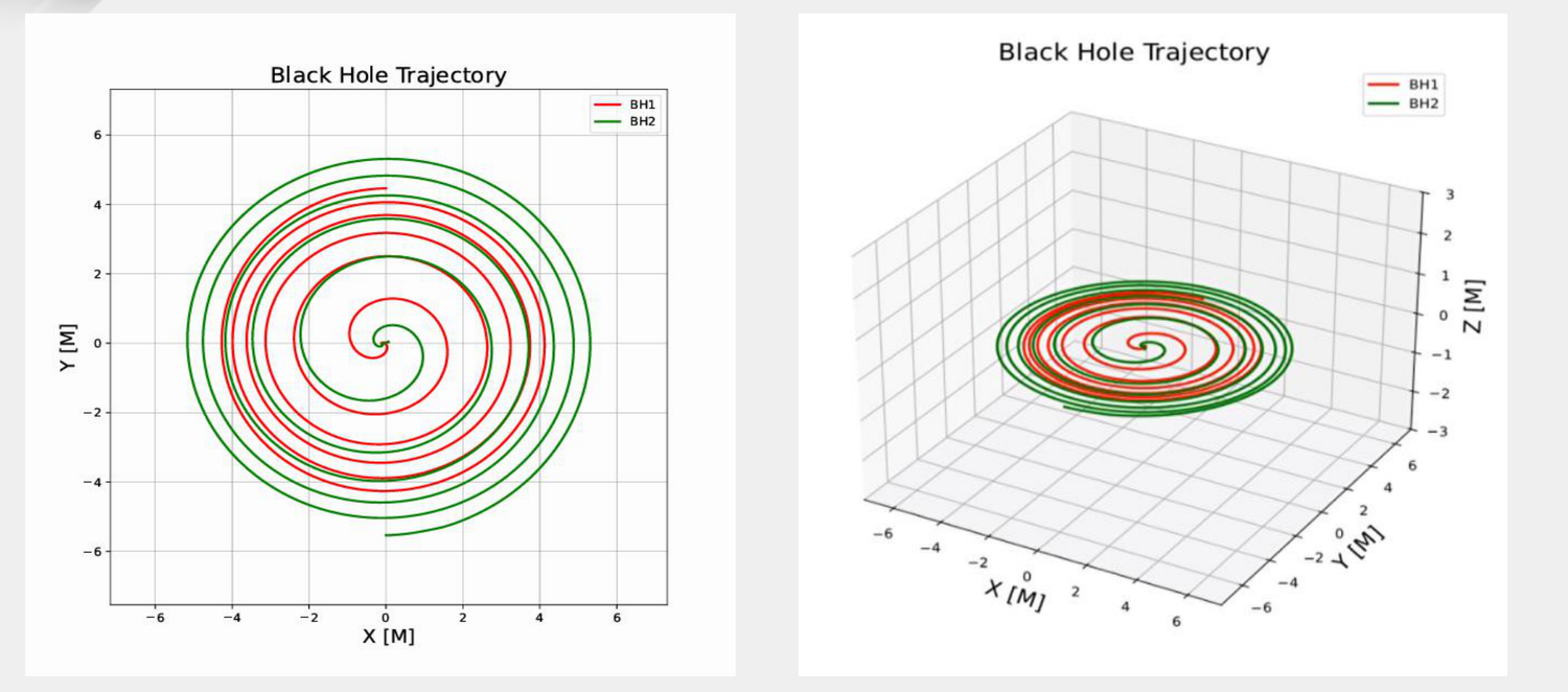
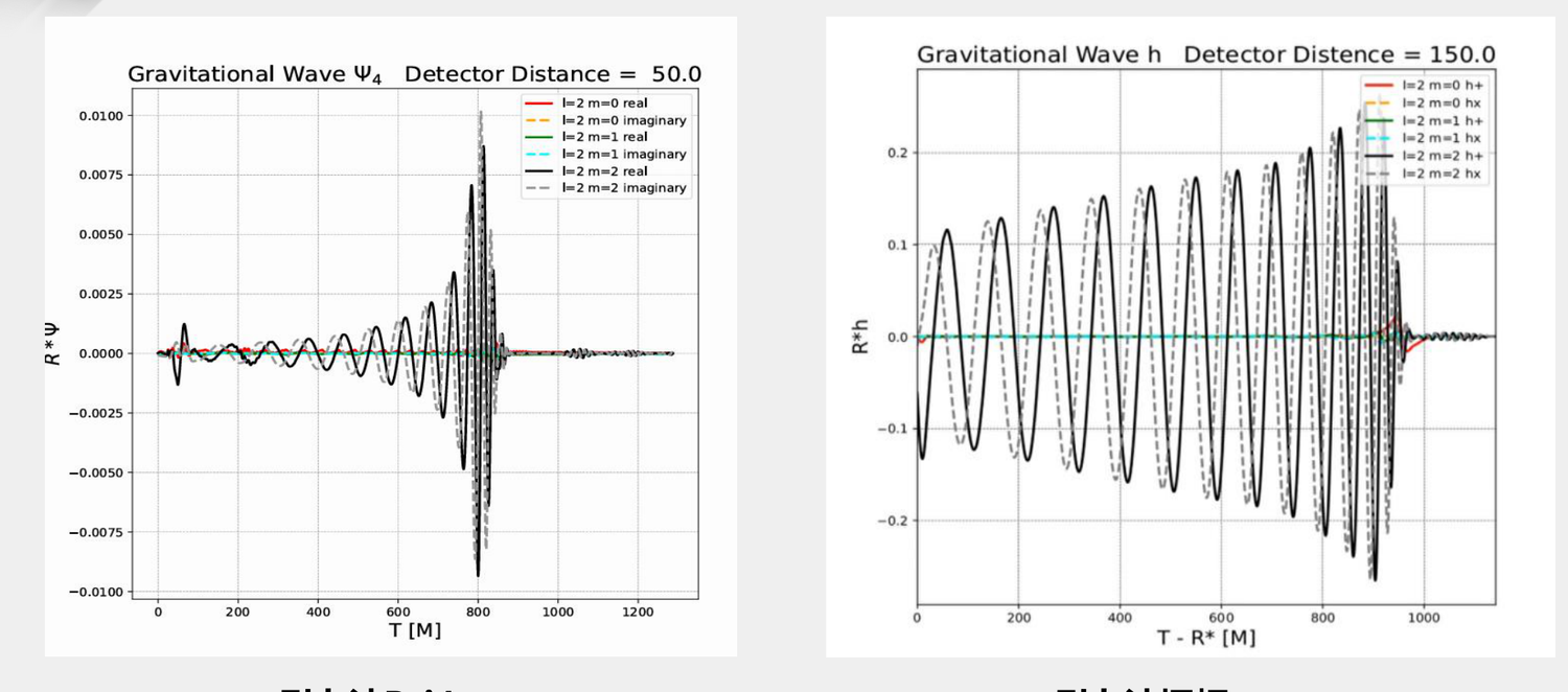
- 黑洞轨迹(2D / 3D)
- Weyl 标量 ψ₄ 与引力波应变 h₊、h×
- Hamilton 约束违反
- ADM 质量与 ADM 动量
- 空间度规共形因子与外曲率迹 TrK 的 2D 热图 / 3D 曲面图
设计理念
界面将「物理问题」与「程序细节」解耦:研究者专注于黑洞系统本身(质量、自旋、轨道、分辨率),构建系统、网格层级、文件组织等技术细节由界面代管。这显著降低了数值相对论模拟的使用门槛,也便于教学与结果复现。
安装与依赖
界面在 Linux 系统下运行,依赖 GCC、NVCC、Python、MPI 以及 numpy、scipy、matplotlib、SymPy、opencv-python 等 Python 库(Ubuntu 22.04 / 24.04 示例):
# 系统依赖(Ubuntu 22.04 / 24.04)
sudo apt-get install gcc gfortran make build-essential
sudo apt-get install python3 python3-pip
sudo apt-get install nvidia-cuda-toolkit        # 可选:GPU 计算
sudo apt-get install openmpi-bin libopenmpi-dev # MPI 并行
sudo apt-get install libopencv-dev python3-opencv
# Python 依赖
pip install numpy scipy matplotlib sympy opencv-python
开源与文献
界面代码已开源(LGPL-2.1 许可),并配套发表论文如下:
- GitHub: github.com/xiaoqu0000/NR-amssncku
- Zenodo: doi:10.5281/zenodo.18674727
- Qiao, C.-K., Zheng, Y. & Cao, Z.-J. A user-friendly Python interface for the numerical relativity code AMSS-NCKU. Astronomy and Computing 55, 101093 (2026). arXiv:2509.21652